Decouple the spatial and temporal components by PCA
Two-Stepreduction.RmdAim
This article explans the code for the subsequent principal component analysis (PCA), proposed in Two-step dimensionality reduction of human mobility data: From potential landscapes to spatiotemporal insights.
Read files of pontials into a single wide dataframe
read each file and make a wide table
file_paths = c(
  "potential_2019_h.csv",
  "potential_2019_w.csv",
  "potential_2021_h.csv",
  "potential_2021_w.csv")

  preprocess <- function(file_path) {
    #read the file
    potential <- read_csv(file_path, col_types=list(zone="c", org_hour="i", dst_hour="i", .default="n"))

    #Add one column that is "weekday2019" or "weekday2021" or "weekday2021" or "holiday2021", depending on if "2019" or "2021" is in the file path, and if "weekday" or "holiday" is in the file path
    potential$day_type <- case_when(
    grepl("2019", file_path) & grepl("_w", file_path) ~ "2019w",
    grepl("2019", file_path) & grepl("_h", file_path) ~ "2019h",
    grepl("2021", file_path) & grepl("_w", file_path) ~ "2021w",
    grepl("2021", file_path) & grepl("_h", file_path) ~ "2021h",
    )

    #combine day_type and org_hour into one column, like "weekday2019-01", with org_hour two digits
    potential$org_hour = paste0(potential$day_type, "-", sprintf("%02d", potential$org_hour))

    #arange by org_hour, and select by zone, org_hour, potential
    potential <- potential %>% arrange(org_hour) %>% select(zone, org_hour, potential)

    #make it a pivot table, where the columns are the zones, the rows are the org_hours, and the values are the potentials
    df_wider <- potential %>% pivot_wider(names_from = zone, values_from = potential)

    #order by weekday2019-00 to weekday2019-23, then holiday2019-00 to holiday2019-23, then weekday2021-00 to weekday2021-23, then holiday2021-00 to holiday2021-23
    df_wider$org_hour <- factor(df_wider$org_hour, levels = c(paste0("2019w-", sprintf("%02d", 0:23)),
                                                              paste0("2019h-", sprintf("%02d", 0:23)),
                                                              paste0("2021w-", sprintf("%02d", 0:23)),
                                                              paste0("2021h-", sprintf("%02d", 0:23))))
    return(df_wider)
  }

# apply the function to all the files, and combine them into one dataframe
df_wider_all <- map_dfr(file_paths, preprocess)
head(df_wider_all)
#> # A tibble: 6 × 1,319
#>   org_hour `533903665` `533903865` `533904805` `533904825` `533904845`
#>   <fct>          <dbl>       <dbl>       <dbl>       <dbl>       <dbl>
#> 1 2019h-00     -0.176       0.0961  -0.229       -0.116         0.191
#> 2 2019h-01     -0.0538     -0.0630  -0.163        0.0925        0.0965
#> 3 2019h-02     -0.148       0.119   -0.0000435   -0.000129     -0.0462
#> 4 2019h-03     -0.0992      0.108   -0.126       -0.0582       -0.111
#> 5 2019h-04     -0.0655      0.0141  -0.0367       0.170         0.153
#> 6 2019h-05      0.0960     -0.213   -0.462       -0.299        -0.206
#> # ℹ 1,313 more variables: `533904885` <dbl>, `533912065` <dbl>,
#> #   `533912485` <dbl>, `533912685` <dbl>, `533913005` <dbl>, `533913065` <dbl>,
#> #   `533913085` <dbl>, `533913205` <dbl>, `533913225` <dbl>, `533913245` <dbl>,
#> #   `533913265` <dbl>, `533913405` <dbl>, `533913425` <dbl>, `533913445` <dbl>,
#> #   `533913465` <dbl>, `533913485` <dbl>, `533913625` <dbl>, `533913645` <dbl>,
#> #   `533913665` <dbl>, `533913685` <dbl>, `533913825` <dbl>, `533913845` <dbl>,
#> #   `533913865` <dbl>, `533913885` <dbl>, `533914005` <dbl>, …
Make it into a matrix
m = as.matrix(df_wider_all %>% select(-org_hour))Principle Component Analysis (PCA)
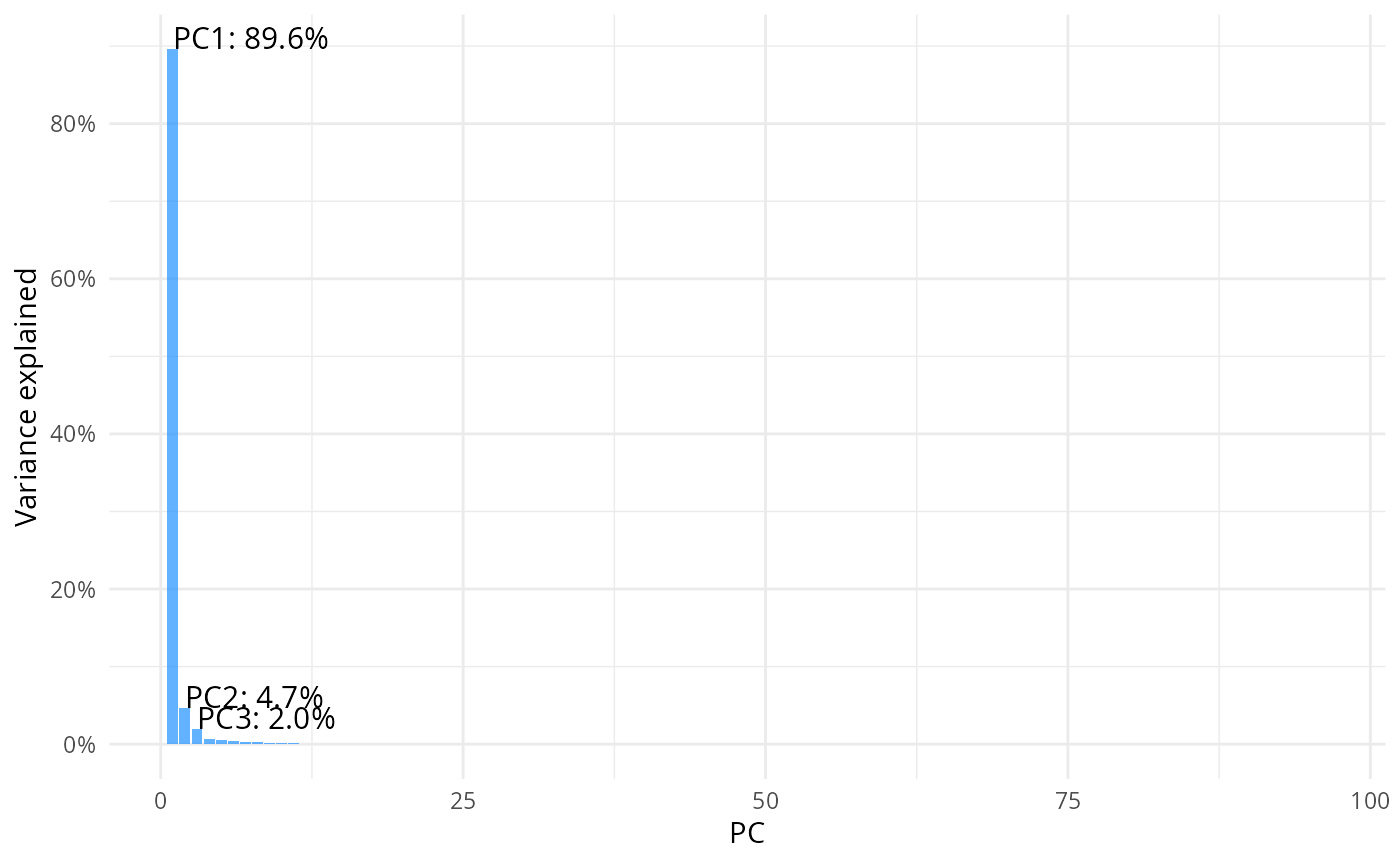
result = prcomp(m, center=T, scale=F)Scree plot
pcs = tidy(result, "pcs")
top3 <- pcs %>% filter(PC %in% 1:3)
ggplot(data = pcs, aes(x=PC, y=percent))+
geom_col(fill="dodgerblue", alpha=0.7) + theme_minimal() +
    scale_y_continuous(labels=scales::label_percent(), breaks = scales::breaks_pretty(n=6))+
    labs(y= "Variance explained")+
    geom_text(
    data = top3,
    aes(
      x = PC,
      y = percent,
      label = paste0("PC", PC, ": ", scales::percent(percent))
    ),
    vjust = 0,
    hjust = 0,
    size = 4
  )
Save PCA rotation (basis)
rotation_df <- as.data.frame(result$rotation)
rotation_df$MESH2KM <- rownames(result$rotation)
rotation_df = rotation_df %>% select(MESH2KM, PC1,PC2,PC3)
#write_csv(rotation_df, "tmp/prc_basis.csv")
head(rotation_df)
#>             MESH2KM          PC1           PC2          PC3
#> 533903665 533903665 -0.007638106  0.0081861818  0.022110372
#> 533903865 533903865 -0.008130319 -0.0092918304 -0.009184783
#> 533904805 533904805 -0.020939566  0.0048591637  0.025925711
#> 533904825 533904825 -0.010935582  0.0034375189  0.003985321
#> 533904845 533904845 -0.020297286  0.0047228773  0.010225484
#> 533904885 533904885 -0.030118096  0.0007656441  0.019902749
Plot temporal evolution of the PC1, PC2 and PC3
augmented_data = augment(result, data = df_wider_all)

# keep only the columns that start with a dot and also the org_hour column, rename the columns to remove the ".fitted" part
augmented_data = augmented_data %>% select(starts_with("."), org_hour) %>% rename_all(~str_remove(., "\\.fitted"))
# split the org_hour column into two columns, one for the day type and one for the hour
augmented_data = augmented_data %>% separate(org_hour, c("day_type", "hour"), sep="-") %>% relocate(day_type, hour) %>% select(-.rownames)
head(augmented_data)
#> # A tibble: 6 × 98
#>   day_type hour     PC1     PC2    PC3     PC4    PC5    PC6   PC7    PC8
#>   <chr>    <chr>  <dbl>   <dbl>  <dbl>   <dbl>  <dbl>  <dbl> <dbl>  <dbl>
#> 1 2019h    00    -8.78  -7.10   -0.613 -3.43    1.28  -0.506 1.20  2.93
#> 2 2019h    01    -2.11  -4.24   -1.32  -2.45    0.478  0.728 1.37  1.88
#> 3 2019h    02    -0.508 -2.28   -1.38  -1.72   -0.319  0.500 1.09  1.52
#> 4 2019h    03     0.290 -1.53   -1.02  -1.24   -0.905  0.378 0.838 1.13
#> 5 2019h    04     2.02   0.0869 -0.984 -0.628  -2.12   0.405 0.574 0.609
#> 6 2019h    05    12.6    3.62   -3.46  -0.0853 -1.97   1.00  0.272 0.0869
#> # ℹ 88 more variables: PC9 <dbl>, PC10 <dbl>, PC11 <dbl>, PC12 <dbl>,
#> #   PC13 <dbl>, PC14 <dbl>, PC15 <dbl>, PC16 <dbl>, PC17 <dbl>, PC18 <dbl>,
#> #   PC19 <dbl>, PC20 <dbl>, PC21 <dbl>, PC22 <dbl>, PC23 <dbl>, PC24 <dbl>,
#> #   PC25 <dbl>, PC26 <dbl>, PC27 <dbl>, PC28 <dbl>, PC29 <dbl>, PC30 <dbl>,
#> #   PC31 <dbl>, PC32 <dbl>, PC33 <dbl>, PC34 <dbl>, PC35 <dbl>, PC36 <dbl>,
#> #   PC37 <dbl>, PC38 <dbl>, PC39 <dbl>, PC40 <dbl>, PC41 <dbl>, PC42 <dbl>,
#> #   PC43 <dbl>, PC44 <dbl>, PC45 <dbl>, PC46 <dbl>, PC47 <dbl>, PC48 <dbl>, …
pickup weekdau in 2019
filtered_data <- augmented_data %>% filter(day_type == "2019w")
head(filtered_data)
#> # A tibble: 6 × 98
#>   day_type hour     PC1    PC2    PC3    PC4    PC5    PC6     PC7   PC8     PC9
#>   <chr>    <chr>  <dbl>  <dbl>  <dbl>  <dbl>  <dbl>  <dbl>   <dbl> <dbl>   <dbl>
#> 1 2019w    00    -6.61  -3.28  -1.20  -2.74  -0.805  1.21  -0.0104 0.665 -0.0368
#> 2 2019w    01    -2.04  -1.76  -1.62  -2.10  -1.24   1.55   0.702  0.161 -0.246
#> 3 2019w    02    -0.458 -0.762 -1.35  -1.17  -1.28   0.797  0.472  0.154 -0.0177
#> 4 2019w    03     0.466 -0.265 -0.898 -0.968 -1.44   0.431  0.439  0.202  0.0560
#> 5 2019w    04     2.99   1.09  -1.14   0.239 -2.55  -0.350  0.813  0.153 -0.222
#> 6 2019w    05    23.5    6.80  -8.44   2.70  -5.56  -2.01   4.10   0.654 -0.551
#> # ℹ 87 more variables: PC10 <dbl>, PC11 <dbl>, PC12 <dbl>, PC13 <dbl>,
#> #   PC14 <dbl>, PC15 <dbl>, PC16 <dbl>, PC17 <dbl>, PC18 <dbl>, PC19 <dbl>,
#> #   PC20 <dbl>, PC21 <dbl>, PC22 <dbl>, PC23 <dbl>, PC24 <dbl>, PC25 <dbl>,
#> #   PC26 <dbl>, PC27 <dbl>, PC28 <dbl>, PC29 <dbl>, PC30 <dbl>, PC31 <dbl>,
#> #   PC32 <dbl>, PC33 <dbl>, PC34 <dbl>, PC35 <dbl>, PC36 <dbl>, PC37 <dbl>,
#> #   PC38 <dbl>, PC39 <dbl>, PC40 <dbl>, PC41 <dbl>, PC42 <dbl>, PC43 <dbl>,
#> #   PC44 <dbl>, PC45 <dbl>, PC46 <dbl>, PC47 <dbl>, PC48 <dbl>, PC49 <dbl>, …
pc1 vs pc2
ggplot(filtered_data, aes(PC1, -PC2, color = as.numeric(hour))) + #PC2 flipped
            geom_path(aes(group = day_type), linewidth = 1) +  # Lines based on hour
            geom_point(size = 4) +  # Points also based on hour
            geom_text_repel(aes(label = hour), min.segment.length = 1, size = 5) +  # Point labels
            scale_color_gradientn(
                colors = c("black", "green", "red", "blue", "black"),  # Custom gradient from night to day
                values = rescale(c(0, 6, 12, 18, 23)),  # Map 0-6 (night) and 18-24 (day) with corresponding colors
                name = "Hour"
            ) +
            theme_minimal() +
            theme(legend.position = "bottom",  # Move legend to the right
                legend.box = "horizontal",  # Ensure vertical arrangement of legend
                legend.title = element_text(face = "bold", margin = margin(r = 50, b = 0)),
                ) +
                guides(
                    color = guide_colorbar(
                    barwidth = 20,
                    barheight = 2,
                    title.position = "left",  # Move the title to the left of the colorbar
                    title.hjust = 0.5,  # Center the title vertically relative to the colorbar
                    label.vjust = 0.5   # Vertically align the labels
                    )
                ) +
            labs(x = "PC1", y = "PC2")
#> Warning: ggrepel: 7 unlabeled data points (too many overlaps). Consider
#> increasing max.overlaps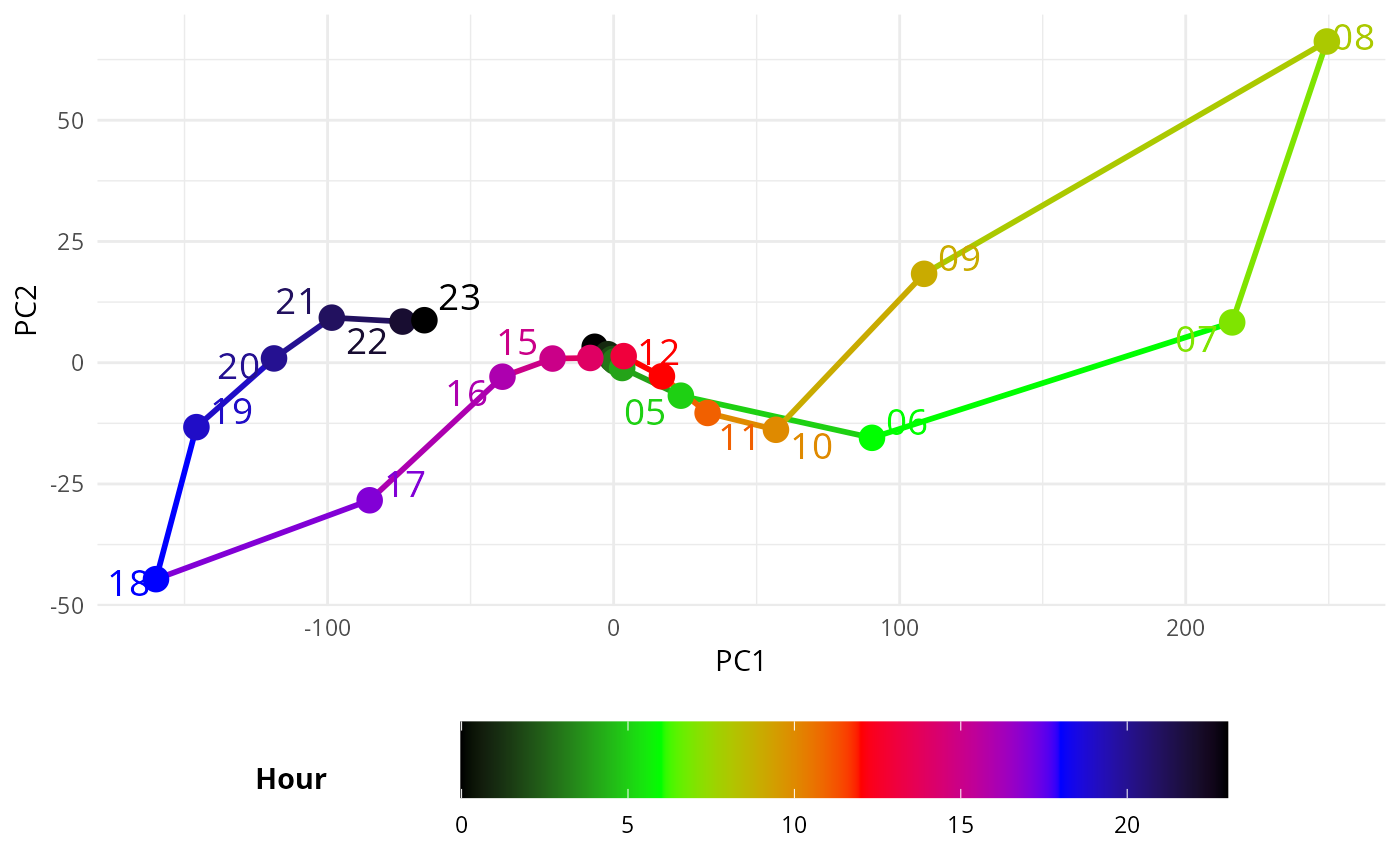
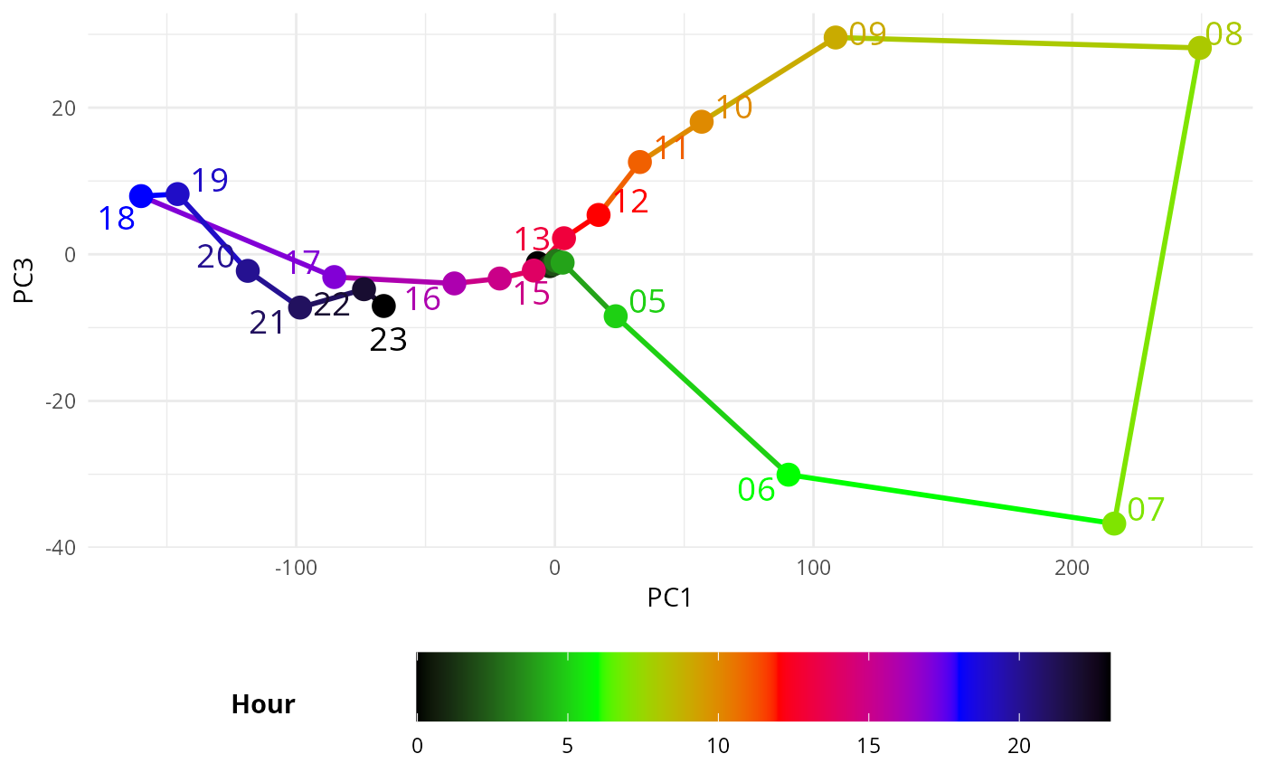
# pc1 vs pc3
ggplot(filtered_data, aes(PC1, PC3, color = as.numeric(hour))) + #PC2 flipped
            geom_path(aes(group = day_type), linewidth = 1) +  # Lines based on hour
            geom_point(size = 4) +  # Points also based on hour
            geom_text_repel(aes(label = hour), min.segment.length = 1, size = 5) +  # Point labels
            scale_color_gradientn(
                colors = c("black", "green", "red", "blue", "black"),  # Custom gradient from night to day
                values = rescale(c(0, 6, 12, 18, 23)),  # Map 0-6 (night) and 18-24 (day) with corresponding colors
                name = "Hour"
            ) +
            theme_minimal() +
            theme(legend.position = "bottom",  # Move legend to the right
                legend.box = "horizontal",  # Ensure vertical arrangement of legend
                legend.title = element_text(face = "bold", margin = margin(r = 50, b = 0)),
                ) +
                guides(
                    color = guide_colorbar(
                    barwidth = 20,
                    barheight = 2,
                    title.position = "left",  # Move the title to the left of the colorbar
                    title.hjust = 0.5,  # Center the title vertically relative to the colorbar
                    label.vjust = 0.5   # Vertically align the labels
                    )
                ) +
            labs(x = "PC1", y = "PC3")
#> Warning: ggrepel: 6 unlabeled data points (too many overlaps). Consider
#> increasing max.overlaps