Potential of Human flow (complete graph case) • HodgePotentialHumanFlow

library(HodgePotentialHumanFlow)

Summary

This vignette shows the scalar potential of a commuting flow in London.

Dataset: origin-destination matrix in London

We use a trip dataset from home to workplace in 2011 obtained from UK Data Service. The OD matrix denotes the number of commuters aggregated by the middle layer super output area (MSOA) in the 2011 census. The dataset covers the MSOAs in England and Wales. Here, we selected the trips only among MSOAs in Greater London.

od = read.csv("london.csv") 
head(od)
#>      origin      dest trips
#> 1 E02000001 E02000001  1506
#> 2 E02000001 E02000014     2
#> 3 E02000001 E02000016     3
#> 4 E02000001 E02000025     1
#> 5 E02000001 E02000028     1
#> 6 E02000001 E02000051     1

Hodge-Kodaira decomposition

Here, we apply Hodge-Kodaira decomposition, in which human flow is uniquely decomposed into a potential-driven (gradient) flow and a curl flow (see our paper for details).

First, we consider the net flow of movement from a given OD matrix $M$ : $A = M - M^{\intercal}, \label{eq:netflow}$ where $M^{\intercal}$ denotes the transpose of $M$ . Matrix $A$ is skew-symmetric, that is, $A_{ij} = - A_{ji}$ , and is possibly described by combinatorial gradient of a potential $s$ , given by $(\text{grad}\, s)(i, j) = s_j-s_i.$

Then, we define an optimization problem for potential $s$ : $\begin{equation} \min_s \lVert \text{grad}\ s - A \rVert_2 = \min_s \left[ \sum_{i,j} \left[ (s_j - s_i) - A_{ij} \right]^2 \right]. \label{eq:optimization_problem} \end{equation}$ According to the combinatorial Hodge theory, the space of net flow $\mathcal{A}$ is orthogonally decomposed into two subspaces: $\begin{equation} \mathcal{A} = \text{im}(\text{grad}) \oplus \text{im}(\text{curl}^*), \end{equation}$ where $\text{curl}$ is the combinatorial curl operator and $\text{curl}^*$ is its adjoint operator. Thus, the optimization problem is equivalent to an $l_2$ -projection of $A$ onto im(grad), and the minimal norm solution is given by $\begin{equation} s_i = -\frac{1}{N} \text{div} A = - \frac{1}{N} \sum_{j=1}^N A_{ij}, \label{eq:potential} \end{equation}$ where $s_i$ is the potential at the $i$ th location and $N$ is the number of locations. It is noted that $s_i$ is negative potential ( $s_i=-V_i$ ). This means we observe more trips from a place with lower potential to another with higher potential.

Using this package, the potential is obtained by the following function.

s = HodgePotentialHumanFlow::scalar_potential_on_complete_graph(od)
#> Percentage of gradient flow = 52.71
head(s)
#>        zone    potential
#> 1 E02000001 244.80671414
#> 2 E02000002  -1.22482197
#> 3 E02000003  -1.15462869
#> 4 E02000004  -1.23397762
#> 5 E02000005  -1.93591048
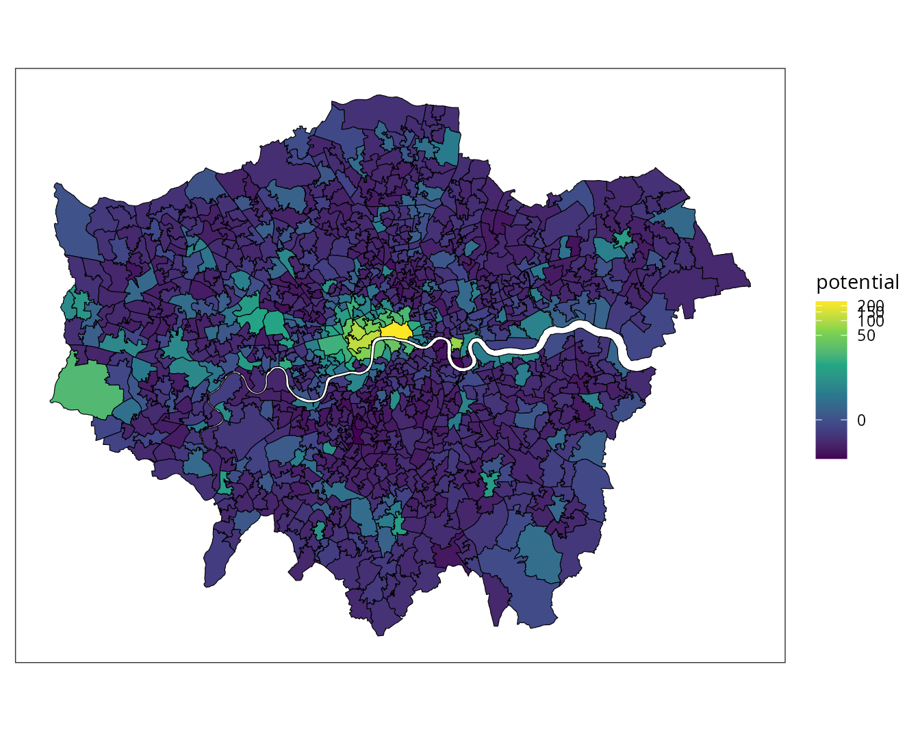
#> 6 E02000007   0.04170905

Plot the obtained potential landscape

The shapefile of the MSOAs is obtained from Office for National Statistics).

suppressWarnings(library(sf))
#> Linking to GEOS 3.13.1, GDAL 3.11.4, PROJ 9.6.0; sf_use_s2() is TRUE
shape = st_read("london.geojson") 
#> Reading layer `MSOA_in_London' from data source 
#>   `/home/aoki/Dropbox/00CurrentProject/HodgePotentialHumanFlow/vignettes/london.geojson' 
#>   using driver `GeoJSON'
#> Simple feature collection with 983 features and 6 fields
#> Geometry type: MULTIPOLYGON
#> Dimension:     XY
#> Bounding box:  xmin: 503569.4 ymin: 155850.7 xmax: 561959.4 ymax: 200934.3
#> Projected CRS: OSGB36 / British National Grid
merged = merge(shape, s, all.x=T, by.x="msoa11cd", by.y="zone")
head(merged)
#> Simple feature collection with 6 features and 7 fields
#> Geometry type: MULTIPOLYGON
#> Dimension:     XY
#> Bounding box:  xmin: 530968.5 ymin: 180510.9 xmax: 551945.7 ymax: 191139.3
#> Projected CRS: OSGB36 / British National Grid
#>    msoa11cd objectid                 msoa11nm                msoa11nmw
#> 1 E02000001        1       City of London 001       City of London 001
#> 2 E02000002        2 Barking and Dagenham 001 Barking and Dagenham 001
#> 3 E02000003        3 Barking and Dagenham 002 Barking and Dagenham 002
#> 4 E02000004        4 Barking and Dagenham 003 Barking and Dagenham 003
#> 5 E02000005        5 Barking and Dagenham 004 Barking and Dagenham 004
#> 6 E02000007        6 Barking and Dagenham 006 Barking and Dagenham 006
#>   st_areashape st_lengthshape    potential                       geometry
#> 1      2897837       9297.742 244.80671414 MULTIPOLYGON (((532155.5 18...
#> 2      2161565       8307.072  -1.22482197 MULTIPOLYGON (((548879.6 19...
#> 3      2141516       9359.992  -1.15462869 MULTIPOLYGON (((548960.4 18...
#> 4      2492948       8476.617  -1.23397762 MULTIPOLYGON (((551551.9 18...
#> 5      1187953       7322.466  -1.93591048 MULTIPOLYGON (((549238.9 18...
#> 6      1735998       7071.096   0.04170905 MULTIPOLYGON (((549420.5 18...

Plot the obtained potential landscape using sf package.

library(ggplot2)
library(viridis)
#> Loading required package: viridisLite
library(scales)
#> 
#> Attaching package: 'scales'
#> The following object is masked from 'package:viridis':
#> 
#>     viridis_pal
ggplot(data=merged, aes(fill=potential)) + geom_sf(color="black", lwd=0.2)  + scale_fill_viridis_c(option="viridis", trans=modulus_trans(0)) + theme_bw() + theme(axis.title = element_blank(), axis.ticks = element_blank(), axis.text = element_blank(),panel.grid.major = element_line(colour = "transparent"))