Potential of Human flow (general graph case)

Tutorial: Potential of Human flow (general graph case)

This tutorial demonstrates how to detect significant sinks and sources of human flow according to the scalar potential in the case of the Tokyo metropolitan area.

Dataset: origin-destination matrix in Tokyo with trip distance

We used a dataset from the person-trip surveys conducted in 2018 in the Tokyo metropolitan area, which is publicly available from the Tokyo Metropolitan Region Transportation Planning Commission.

suppressPackageStartupMessages(library(tidyverse))
od = read_csv("tokyo2018.csv",
              col_types=list(trips = "n", road_distance_in_km="n",.default="c")) 
od
#> # A tibble: 377,610 × 4
#>    origin dest  trips road_distance_in_km
#>    <chr>  <chr> <dbl>               <dbl>
#>  1 0011   0010    990                3.24
#>  2 0012   0010   2445                2.00
#>  3 0020   0010   2793                2.81
#>  4 0021   0010      0                2.07
#>  5 0022   0010      0                2.26
#>  6 0023   0010   1692                3.30
#>  7 0024   0010   1318                4.25
#>  8 0030   0010   2525                4.65
#>  9 0031   0010    893                3.64
#> 10 0032   0010   1426                8.81
#> # ℹ 377,600 more rows

The first two columns indicate the origin and destination zones, representing the geographical zone code defined by the Tokyo Metropolitan Region Transportation Planning Commission. The trips column shows the number of trips. We added the road_distance_in_km column showing the trip distance from the origin to the destination. This distance is evaluated by the road distance between the centroids of the origin and destination zones, calculated by the Open Source Routing Machine (OSRM) based on Open Street Map. The dataset contains 615 unique zones and 615 $\times$ 614 rows (excluding the trips within each zone).

Preprocess: convert the given dataset to net-flow $Y$ on a graph $G(V,E)$

As described in the main text, we denoted the net movements of people as $Y$ on a graph $G(V,E). In the current context, the vertices $V$ correspond to the locations and the edges $E$ are the connections between them.

Distances $d_{ij}$ between locations $i$ and $j$ crucially affect their connections. Trips will be rare for long distances even if the potentials at the endpoints differ. On the other hand, no trips are often observed for short distances. This implies that zero movements happen in two distinct situations. To distinguish the nonexistence of movements based on distance and other factors, we assumed that a pair of locations is connected if its road distance $d_{ij}$ is within a threshold $\theta$ .

We calculate the threshold distance $\theta$ above which trips are rarely observed. We show the cumulative distribution of trip distance $P(X<d)$ as a function of trip distance $d$ . The threshold $\theta$ is determined based on criterion $P(X<\theta) = 0.99$ .

df = od %>% arrange(road_distance_in_km) %>% mutate(cum_trips = cumsum(trips))
df = df %>% mutate( cum_dist = cum_trips / sum(df$trips))
df
#> # A tibble: 377,610 × 6
#>    origin dest  trips road_distance_in_km cum_trips  cum_dist
#>    <chr>  <chr> <dbl>               <dbl>     <dbl>     <dbl>
#>  1 1021   1020    208                1.00       208 0.0000133
#>  2 1020   1021   1643                1.00      1851 0.000118 
#>  3 1022   1021    640                1.04      2491 0.000159 
#>  4 1021   1022    904                1.04      3395 0.000216 
#>  5 3017   3013   1383                1.17      4778 0.000305 
#>  6 3013   3017    829                1.17      5607 0.000358 
#>  7 6023   6021   1820                1.17      7427 0.000474 
#>  8 6021   6023   1035                1.17      8462 0.000540 
#>  9 6061   6060   2601                1.18     11063 0.000705 
#> 10 6060   6061    216                1.18     11279 0.000719 
#> # ℹ 377,600 more rows

# find intersection with threshold
y0 = 0.99
RootLinearInterpolant <- function (x, y, y0 = 0) {
  if (is.unsorted(x)) {
    ind <- order(x)
    x <- x[ind]; y <- y[ind]
  }
  z <- y - y0
  k <- which(z[-1] * z[-length(z)] < 0)
  xk <- x[k] - z[k] * (x[k + 1] - x[k]) / (z[k + 1] - z[k])
  return(xk)
}
thres = RootLinearInterpolant(df$road_distance_in_km, df$cum_dist, y0)

library(ggplot2)
theme_set(theme_minimal())
ggplot(df, aes(x = road_distance_in_km, y=cum_dist) ) +
  geom_line(linewidth=1.3) + 
  xlab("Distance [km]") + 
  ylab("Cumulative distribution, Prob. (X < d)")  + 
  geom_hline(yintercept= y0, color="red", linetype="dashed") +
  annotate("segment", x=thres,xend=thres, y=y0 - 0.1, yend=y0, 
           arrow=arrow(length = unit(2, "mm")) ) + 
  annotate("text", x = thres, y = y0 - 0.15, 
           label=sprintf("%.1fkm", thres),size=3)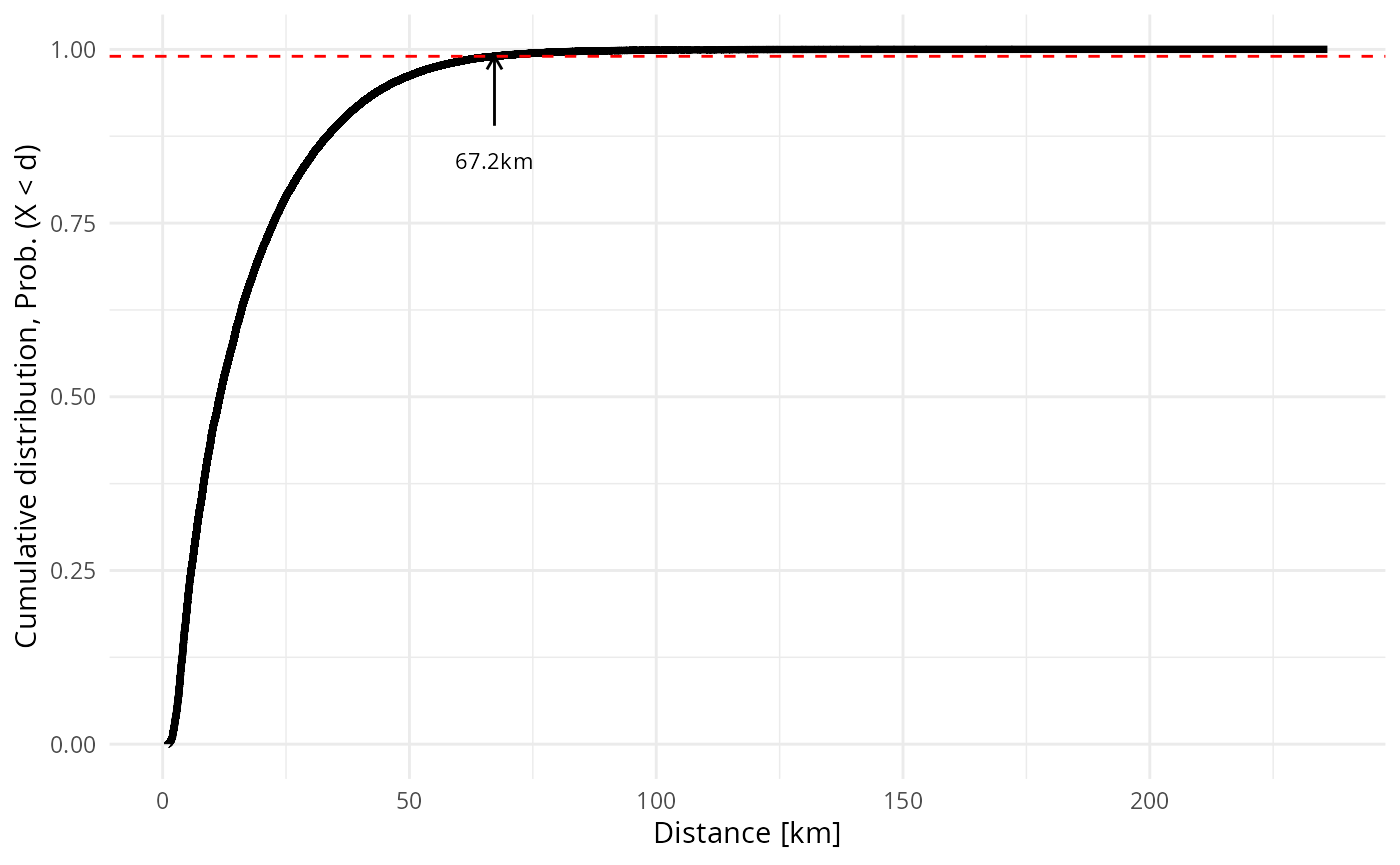

Next, we make net flows between all pairs of locations and select them by $d_{ij} < \theta$ .

od_forward = od 
od_backward = od_forward %>% select(origin,dest,trips) %>% 
  rename(origin_new = dest, dest_new = origin) %>% 
  rename(origin = origin_new, dest = dest_new, back_trips = trips ) %>%
  select(origin, dest, back_trips)


netflow = od_forward %>% left_join(od_backward,by = join_by(origin, dest)) %>%
  filter(origin > dest) %>% mutate(netflow = trips - back_trips) %>% 
  rename(vertex1 = origin, vertex2=dest)

netflow_selected = netflow %>% 
  filter(road_distance_in_km < thres) %>% 
  select(vertex1,vertex2,netflow)

netflow_selected
#> # A tibble: 117,329 × 3
#>    vertex1 vertex2 netflow
#>    <chr>   <chr>     <dbl>
#>  1 0011    0010        990
#>  2 0012    0010       2323
#>  3 0020    0010       2793
#>  4 0021    0010          0
#>  5 0022    0010          0
#>  6 0023    0010       1692
#>  7 0024    0010       1318
#>  8 0030    0010       2525
#>  9 0031    0010        893
#> 10 0032    0010       1426
#> # ℹ 117,319 more rows

Calculate the potential $s$ for the net flow $Y$

The potential is calculated by using function scalar_potential_on_graph in the HodgePotentialHumanFlow package.

library(HodgePotentialHumanFlow)
s = HodgePotentialHumanFlow::scalar_potential_on_graph(netflow_selected)
#> Calculating p-values by monte calro (100000 steps). thread = 32
head(s)
#>   zone potential pvalue_above
#> 1 0011  406.7119            0
#> 2 0012  494.1058            0
#> 3 0020  261.1093            0
#> 4 0021  222.9379            0
#> 5 0022  191.7659            0
#> 6 0023  227.1667            0

The function returns a dataframe with three columns: zone, potential, and $p$ -value. The $p$ -value indicates $P(\hat{s}_i > s_i)$ under the null hypothesis (see the main text for details). The sample number for calculating this pseudo $p$ -value can be specified by option num_samples (default = 1e5).

s = HodgePotentialHumanFlow::scalar_potential_on_graph(netflow_selected, num_samples = 1e5)
#> Calculating p-values by monte calro (100000 steps). thread = 32

We plot the potential on a map using a shapefile publicly available from the Tokyo Metropolitan Region Transportation Planning Commission.

library(sf)
#> Linking to GEOS 3.13.1, GDAL 3.11.4, PROJ 9.6.0; sf_use_s2() is TRUE
map = st_read("tokyo2018.gpkg", quiet=T) 
map = map %>% left_join(s)
#> Joining with `by = join_by(zone)`

library(ggplot2)
library(viridis,quietly = T)
suppressPackageStartupMessages(library(urbnthemes,quietly=T))
library(ggspatial,quietly=T)
suppressPackageStartupMessages(library(scales,quiet = T))


ggplot(data=map, aes(fill=potential)) + 
  geom_sf(color="black", lwd=0.2)  +
  scale_fill_viridis_c(option="viridis", trans=modulus_trans(0.3)) +
  theme_urbn_map(base_family="Helvetica") +
  theme(legend.key.height=unit(1.5,"line")) +
  annotation_scale(location = "bl") + 
  annotation_north_arrow(location = "br", which_north = "grid", 
  style = north_arrow_fancy_orienteering(text_size =0, line_width=0.5))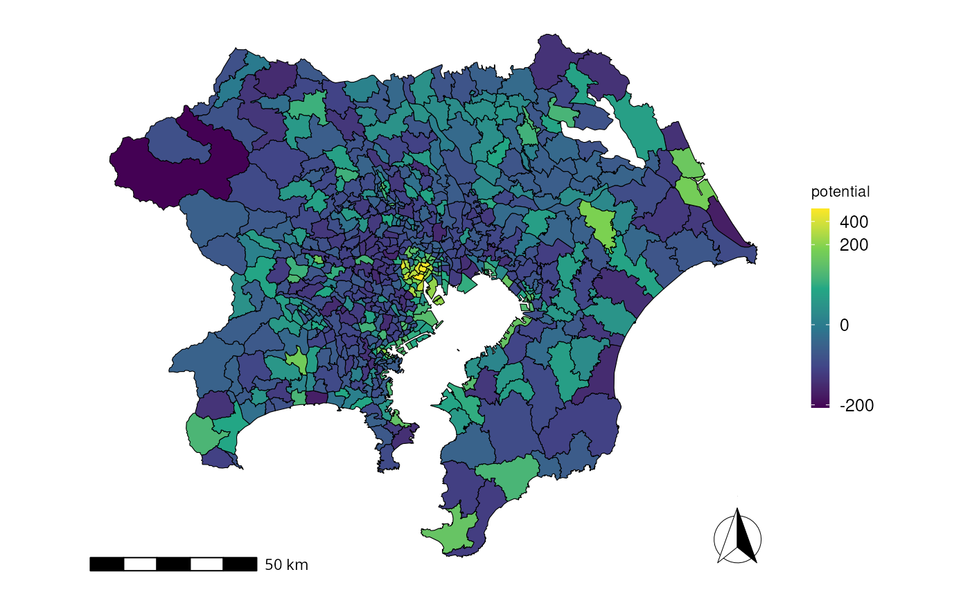

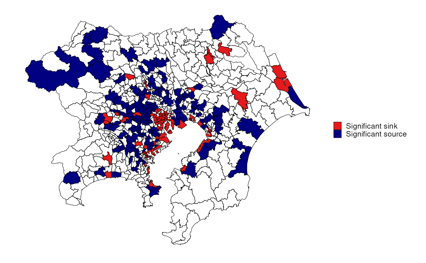
Detect significant sinks and sources

To detect significant sinks for zones with a positive potential, a multiple-comparison test is performed using the $p$ -value under the control of the false discovery rate (FDR), $\alpha (=0.05)$ , with a standard Benjamini-Hochberg procedure. Similarly, for zones with a negative potential, a multiple-comparison test is performed using the $p$ -value of $1 - P(\hat{s}_i > s_i)$ under FDR control.

df_sink= s %>% filter(potential >= 0)
df_sink$pvalue_adj = p.adjust(df_sink$pvalue_above, method="fdr")
df_source= s %>% filter(potential < 0)
df_source$pvalue_adj = p.adjust(1 - df_source$pvalue_above, method="fdr")
df = rbind(df_sink, df_source)

library(sf)
alpha = 0.05
map = st_read("tokyo2018.gpkg", quiet=T) 
map = map %>% left_join(df) %>% rowwise() %>% 
   mutate(type = case_when(
                      potential >= 0 & pvalue_adj < alpha ~ "Significant sink",
                      potential < 0 & pvalue_adj < alpha ~ "Significant source",
   ))
#> Joining with `by = join_by(zone)`
ggplot(data=map, aes(fill=type)) + 
  geom_sf(color="black", lwd=0.2)  +
  theme_urbn_map(base_family="Helvetica") +
  scale_fill_manual(values = c("#e41a1c","navyblue"),na.translate = F) +
  theme(legend.title=element_blank())

Tutorial: Potential of Human flow (general graph case)

Dataset: origin-destination matrix in Tokyo with trip distance

Preprocess: convert the given dataset to net-flow YY on a graph G(V,E)G(V,E)

Calculate the potential ss for the net flow YY

Detect significant sinks and sources

Preprocess: convert the given dataset to net-flow $Y$ on a graph $G(V,E)$

Calculate the potential $s$ for the net flow $Y$